First data analysis with Python in a Jupyter Notebook

This quick tutorial will show you how to use Jupyter Notebooks within Positron. We will:

• Install Positron
• Create a Python project with its own virtual environment
• Install the packages we need for our analysis
• Open a Jupyter Notebook
• Explore some data

Install Positron

Positron is a free and source available code editor for data scientists. To install Positron on your computer, visit our download page and click Download.

The Positron download page

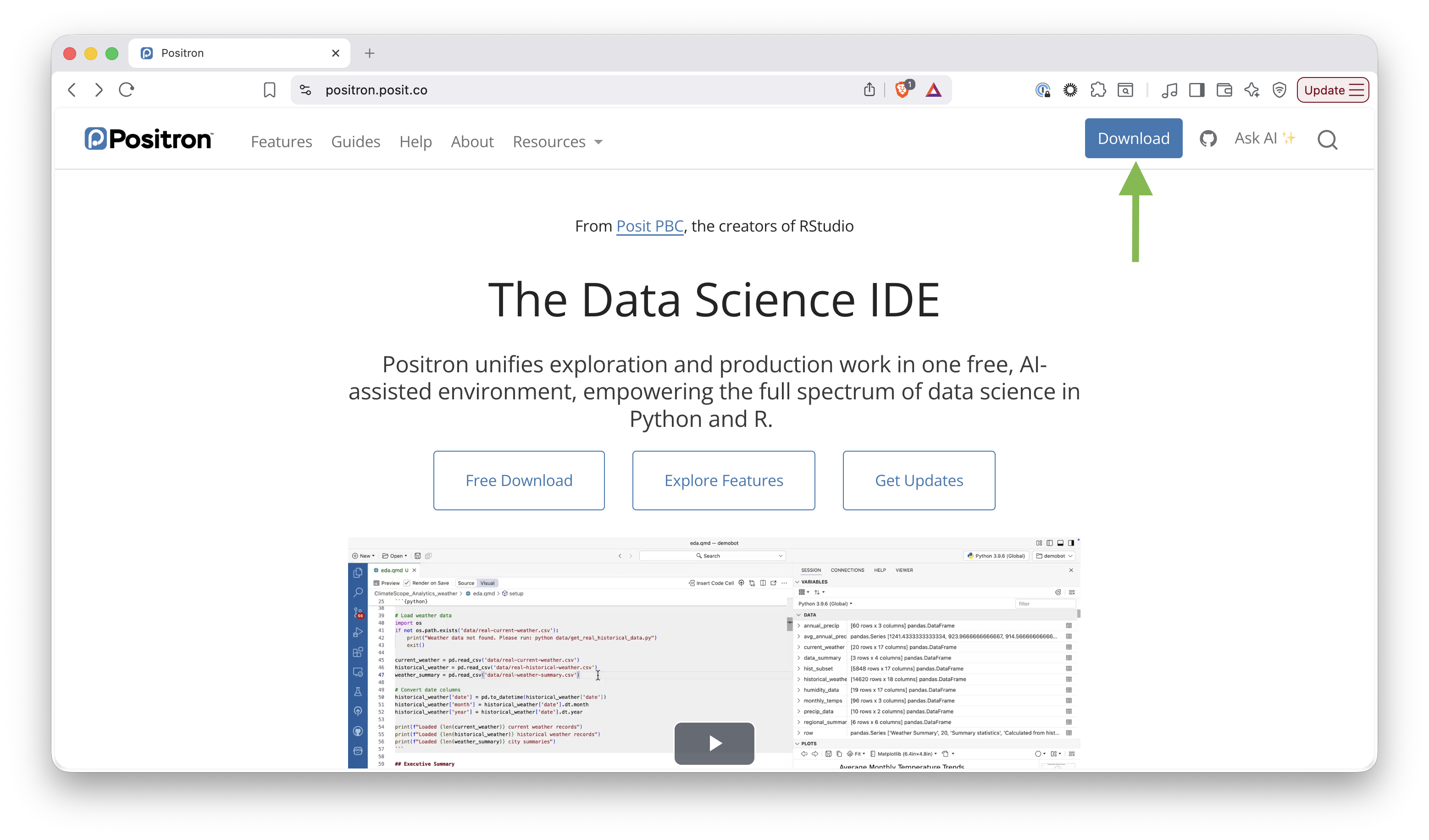
Follow the instructions to install Positron.

Make a Python environment

Python users typically create a project folder for each analysis they do. This keeps all the files for that project organized in one place. Each project also has its own virtual environment, which is a self-contained Python environment that has its own set of packages installed. This allows you to have different versions of packages for different projects without conflicts.

To create a project folder with its own virtual environment in Positron, follow these steps:

1. Open Positron
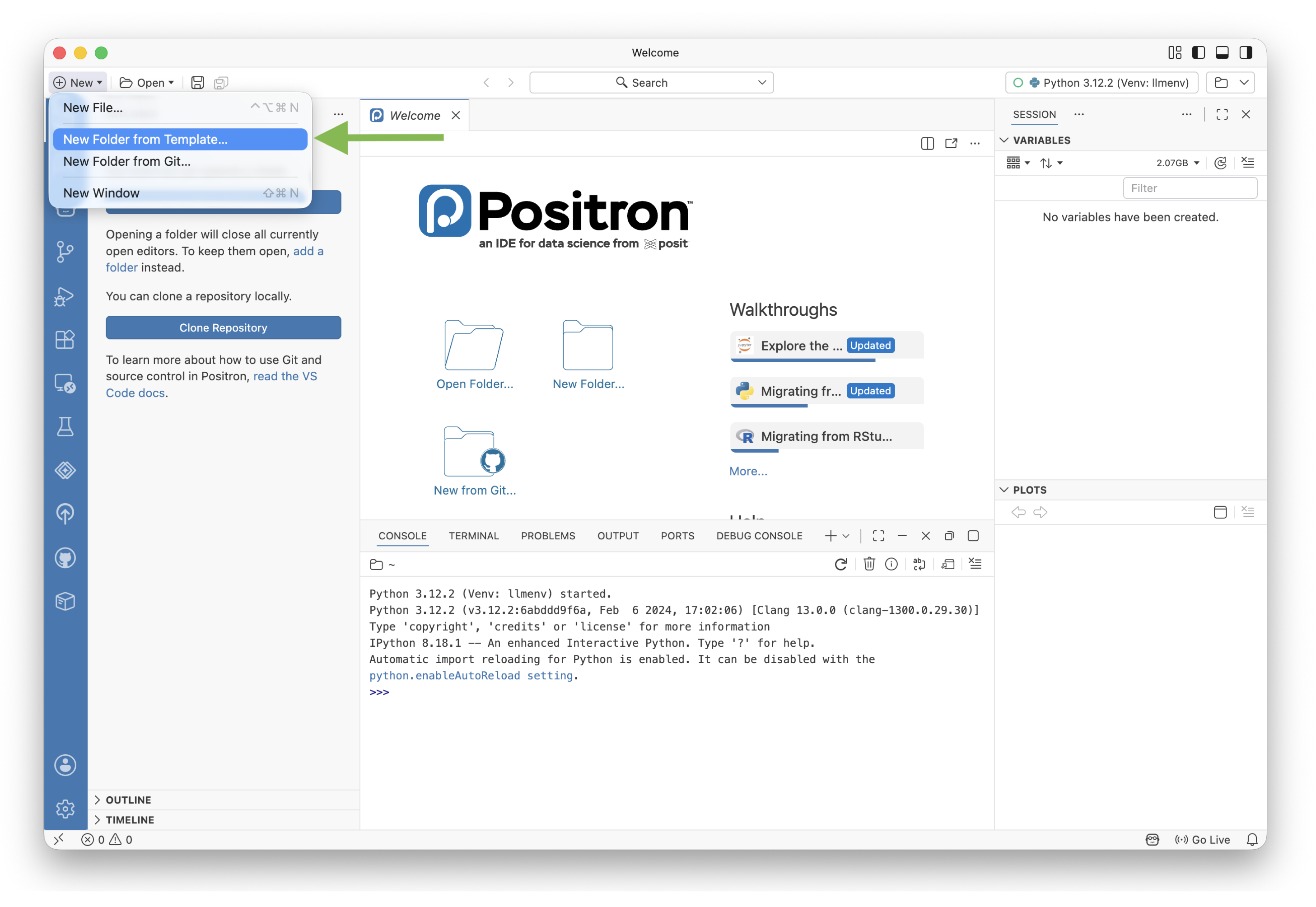
2. Select New > New Folder from Template

New Folder from Template in the File menu

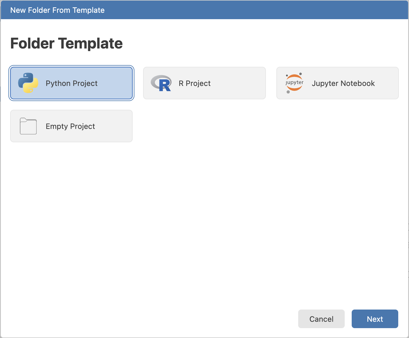
3. Select Python Project from the list of templates

Python Project template

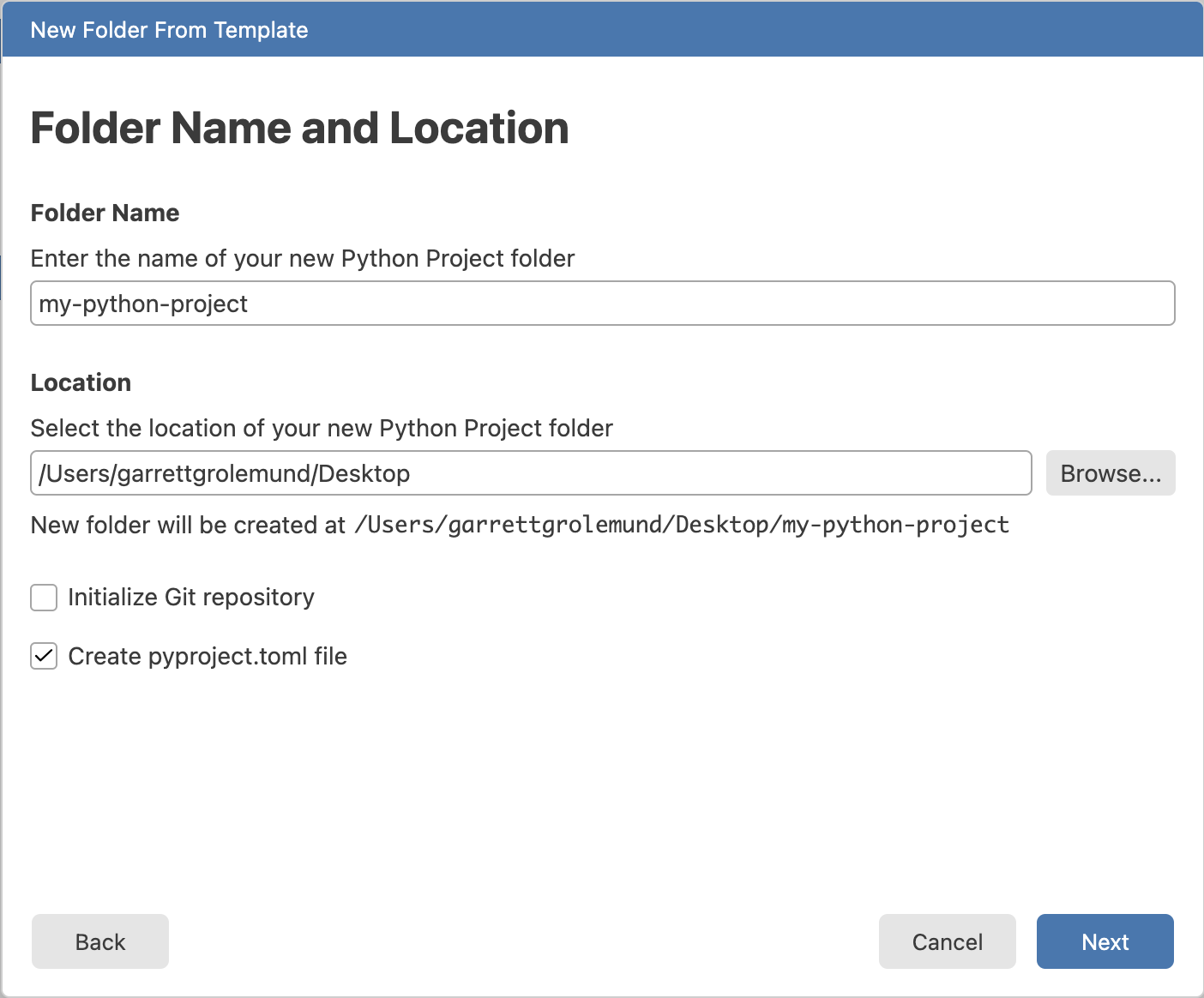
4. Select a location for your project folder and give it a name. Then select Create a pyproject.toml file. This file keeps track of the packages you install in your virtual environment. Then click Next.

Create Python Project dialog

The next screen will help you set up your Python environment.

1. Choose whether to create a new virtual environment or to use an existing environment. For this tutorial, we will create a new virtual environment.

2. Select a tool to build your environment. We recommend uv, but you can also use pip or conda.

3. Give your environment a name. Python users typically choose .venv as the name for their virtual environments, but you can choose any name you like.

4. Select a Python version to use for your environment. We recommend using the latest stable version of Python.

Create Python Environment dialog

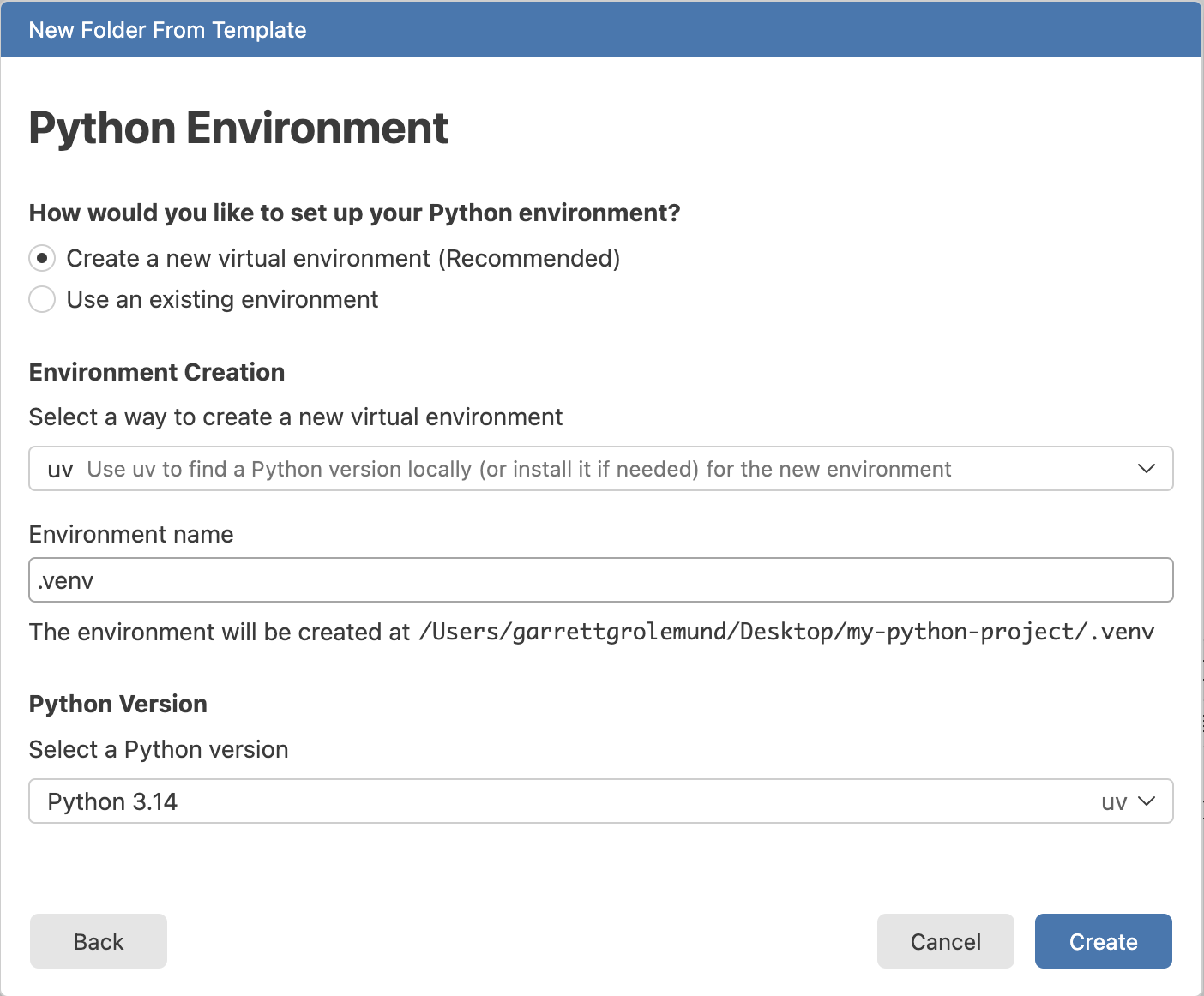
Once you have made your selections, click Create. Positron creates the project folder and sets up the virtual environment for you.

Install packages

Now that we have an environment set up, we need to install the packages we will use for our analysis. For this tutorial, we will use the pandas and plotnine packages.

plotnine is a Python package for creating complex and informative visualizations. It is based on the grammar of graphics, which is a powerful and flexible way to create visualizations.

To install pandas and plotnine, navigate to the Terminal in Positron (View > Terminal). When Positron opened our project, it navigated the Terminal to our project folder and activated the virtual environment we created.

Important

The name of your environment appears in parentheses at the beginning of the terminal prompt. If you do not see it, activate the environment with the command source .venv/bin/activate (replace .venv with the name of your environment if you chose a different name).

We recommend running the following command to install the packages:

uv add pandas plotnine

uv add installs the package and adds it to your pyproject.toml file so that you can keep track of the packages you have installed in your environment.

This is what it looks like to set up a new Python project in Positron:

Open a Jupyter Notebook

Now that we have our environment set up and the packages we need installed, we can open a Jupyter Notebook to start our analysis.

To open a Jupyter Notebook in Positron:

1. Select New > New File
2. Select Jupyter Notebook from the list of file types

New Jupyter Notebook file

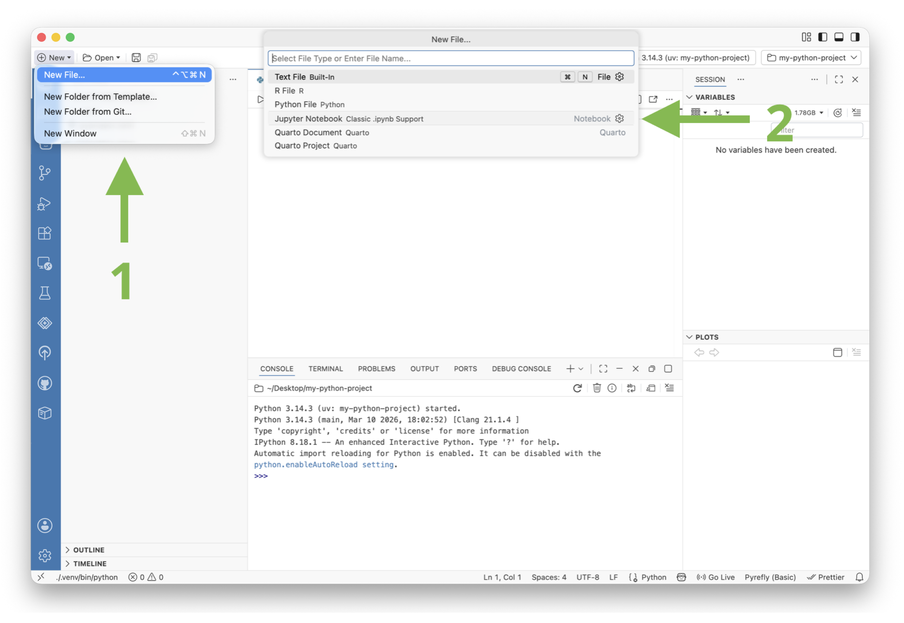
This creates a new Jupyter Notebook file in your project folder and opens it in the editor. You can now start writing code in the notebook and running it to see the results.

You can also open an existing Jupyter Notebook by selecting it in the File Explorer. Positron recognizes that it is a Jupyter Notebook and opens it in the editor.

Above the notebook, Positron adds a toolbar with buttons to run your code, add new cells, select a different kernel, and more. You can use these buttons to interact with your notebook.

When you first open your notebook, it uses your active environment as its kernel. The Positron toolbar also updates to show your Jupyter Notebook as the active session. This means that the rest of the IDE reflects the state of your notebook. For example, the Variables pane shows the variables in your notebook’s kernel.

Explore some data

Now that we have our Jupyter Notebook open, we can start exploring some data. For this tutorial, we will use the mpg dataset, which is a built-in dataset in the plotnine package. To load the dataset:

Point to the area where you would like to insert a new cell and click + Code.

Then paste the following code into the cell and click Run:

from plotnine.data import mpg

This loads the mpg dataset into your notebook’s kernel. Notice that the Variables pane to the right of the notebook shows a new variable called mpg. This variable contains the dataset we just loaded.

The mpg dataset in the Variables pane

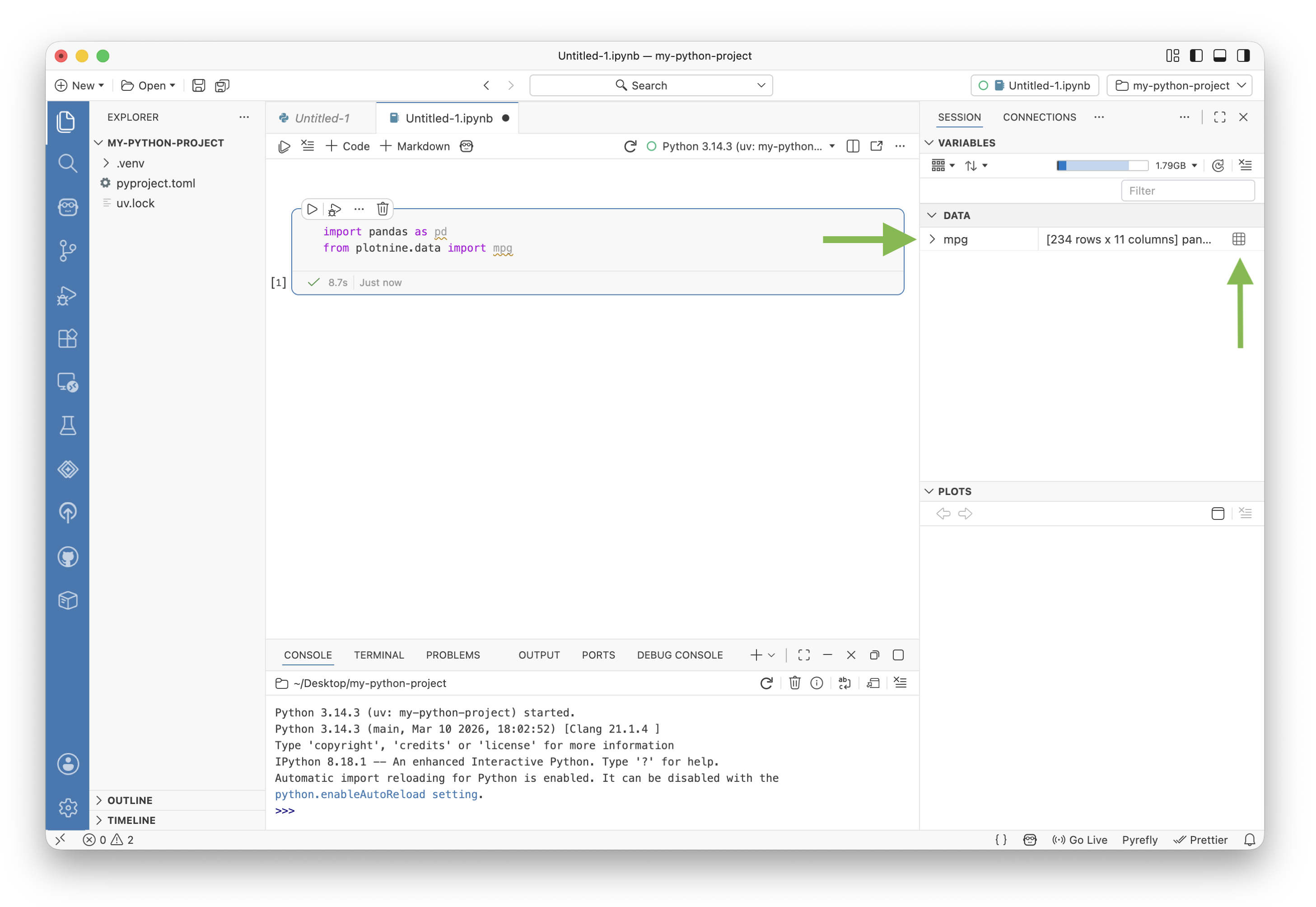
You can use the Variables pane to explore the columns in the dataset. Or you can click the grid-like icon to open the dataset in the Positron Data Explorer.

The Data Explorer allows you to sort and filter the data, as well as view summary statistics. If you would like to recreate a filter, click Convert to Code to copy the code for that filter to your clipboard. You can then paste that code into a cell in your notebook to run it.

We will use the following code to filter mpg to only rows where year is 2008:

mpg_2008 = mpg[mpg['year'] == 2008]

The video below shows how to use the Data Explorer to filter the data and copy the code for that filter to a notebook cell.

Next we will visualize the relationship between the engine displacement (displ) and the miles per gallon (mpg) for cars from 2008 using plotnine:

from plotnine import *

(ggplot(mpg_2008, aes(x='displ', y='hwy'))
 + geom_jitter(aes(color='class'))
 + geom_smooth(method='lm', se=False)
    + labs(title='MPG: Displacement vs Highway Mileage',
            x='Displacement (liters)',
            y='Highway Mileage (mpg)'))

We will also add a code cell that returns a formatted table of the average highway mileage for each class of car:

(mpg_2008.groupby('class')['hwy']
 .mean()
 .reset_index()
 .sort_values(by='hwy', ascending=False))

Finally, we will place a markdown cell with a title at the top of the notebook. To do this, point to the area where you would like to insert the new cell and click + Markdown.

Watch the video below to see these steps in action:

To test that the notebook runs correctly, click Clear Outputs in the toolbar to clear all of the outputs from the cells. Next, click Restart Kernel to create a fresh session. Then click Run All to run all of the cells in order. The plot and the table appear as outputs from the cells.

The entire process looks like this:

Save your notebook

To save your notebook, use the keyboard shortcut . This saves your notebook to your project folder, where it appears in the File Explorer in the left sidebar.

Saving a notebook in Positron

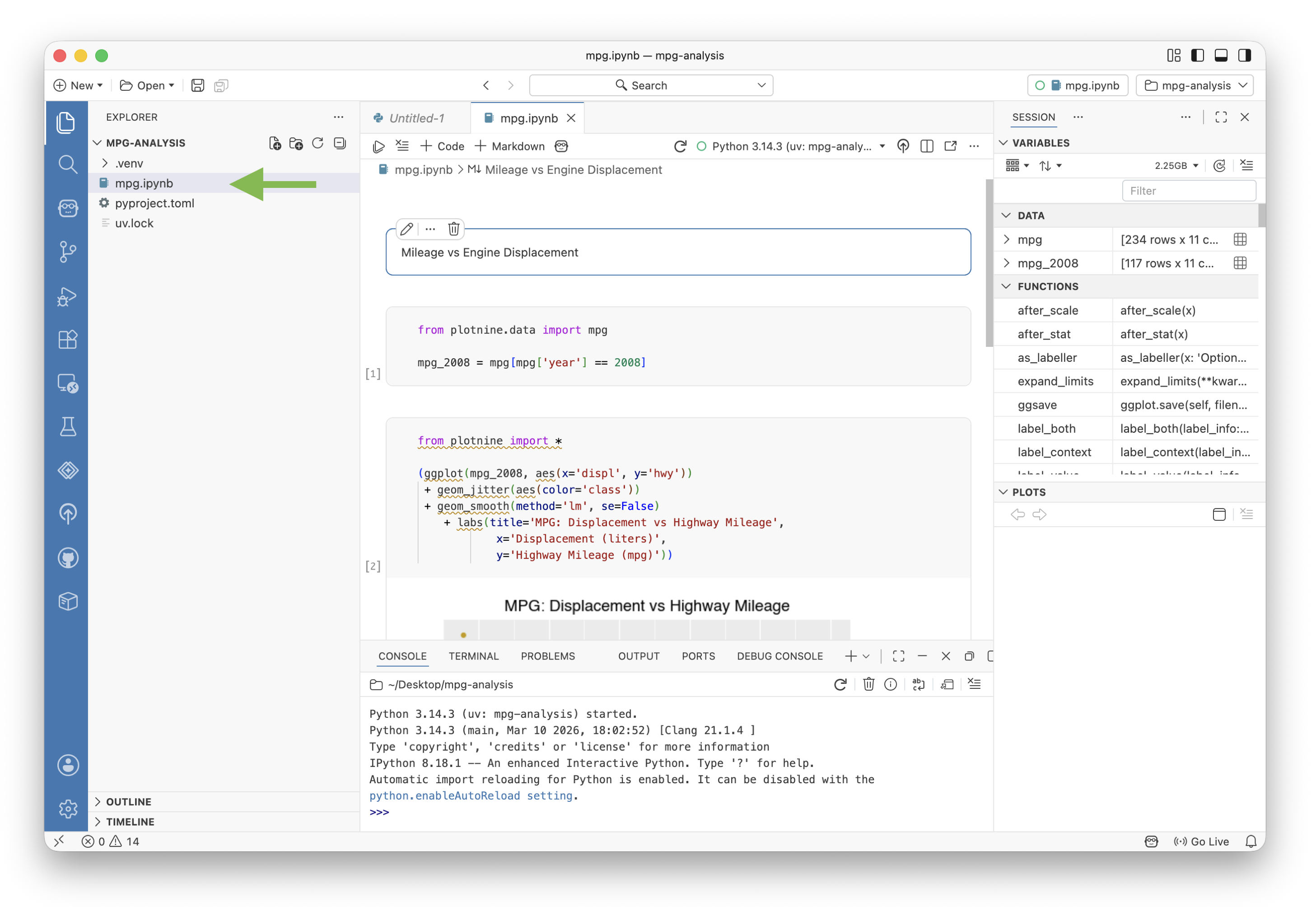
If you have Git set up for your project, you can use the Git pane in Positron to commit and push your notebook to a remote repository like GitHub. This is a great way to share your notebook with others or to keep a backup of your work.

Learn more about using Git in Positron.

Conclusion

Congratulations! You have successfully set up a Python environment in Positron, installed the packages you need, and explored some data in a Jupyter Notebook.

NoteNext steps

To keep going, explore the Guides for in-depth documentation on everything Positron can do.